
For the second post, we will connect the dots in kinematic materials (forward/differential/inverse).
Notations
\[\begin{aligned} q &= \text{Joint state, position} \\ \dot{q} &= \text{Joint velocity} \\ \ddot{q} &= \text{Joint acceleration} \\ X^G &= f_{kin}^G(q) \end{aligned}\]Forward kinematics is a function ($f_{kin}$) that specify the joint angles ($q$), where will the gripper ($X$) end up. However, we usually have a target position to reach which will introduce a difference between the current position vs the target position. That motivates us to calculate the Jacobian of $X^G$
\[\begin{equation}dX^G = \dfrac{\partial{f_{kin}^G(q)}}{\partial q} dq = J^G(q)dq. \end{equation}\]which tells us how far does the gripper move given the joint configuration differences. Then if we have a trajectory of $q$, we will be able to figure out the final position of the gripper:
\[\int_t J^G(q) dq = \int_t J^G(q) \dot{q} dt\]The above equation give a practical meaning that the final position of the gripper is given by the intergral of joint velocities mapped by Jacobian calculated from $X^G$.
Example: Planar 2-joint arm
The $X_G$ is given by
\[\begin{bmatrix} L_1 \cos\theta_1 + L_2 \cos(\theta_1 + \theta_2) \\ L_1 \sin\theta_1 + L_2 \sin(\theta_1 + \theta_2) \end{bmatrix}\]while $J_G$ is given by
\[J_G(q) = \begin{bmatrix} \dfrac{\partial x_G}{\partial \theta_1} & \dfrac{\partial x_G}{\partial \theta_2} \\ \dfrac{\partial y_G}{\partial \theta_1} & \dfrac{\partial y_G}{\partial \theta_2} \end{bmatrix} = \begin{bmatrix} L_1 \sin\theta_1 - L_2 \sin(\theta_1 + \theta_2) & L_2 \sin(\theta_1 + \theta_2) \\ L_1 \cos\theta_1 + L_2 \cos(\theta_1 + \theta_2) & L_2 \cos(\theta_1 + \theta_2) \end{bmatrix}\]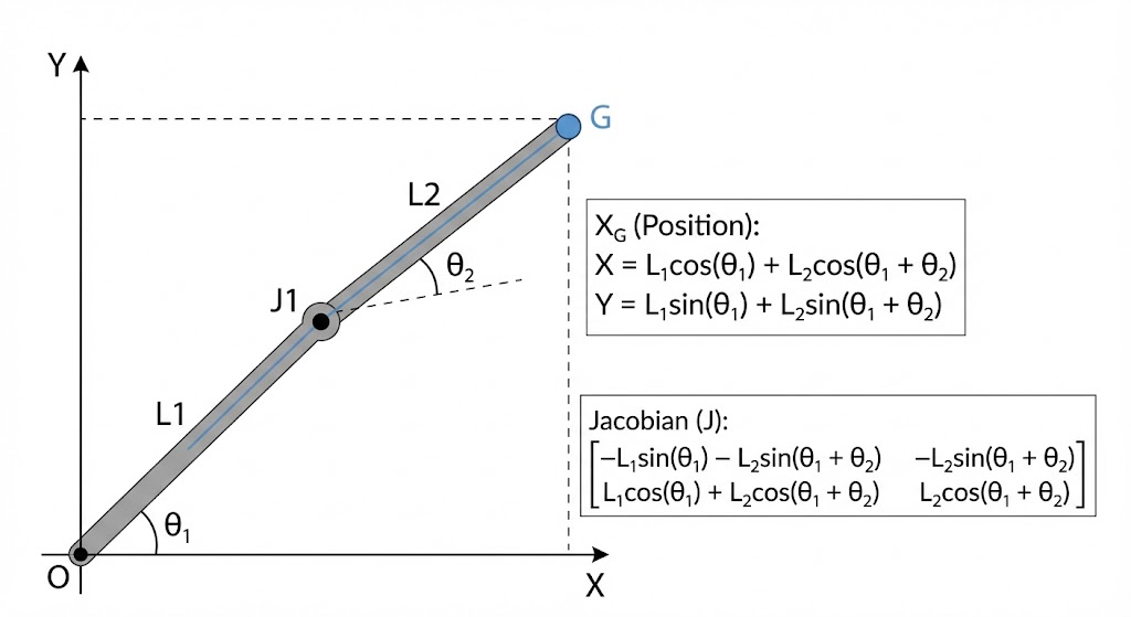
import numpy as np

def fk_2link(q, l1=1.0, l2=1.0):
    q1, q2 = q
    x = l1*np.cos(q1) + l2*np.cos(q1 + q2)
    y = l1*np.sin(q1) + l2*np.sin(q1 + q2)
    return np.array([x, y])

def jacobian_2link(q, l1=1.0, l2=1.0):
    q1, q2 = q
    J = np.array([
        [-l1*np.sin(q1) - l2*np.sin(q1 + q2), -l2*np.sin(q1 + q2)],
        [ l1*np.cos(q1) + l2*np.cos(q1 + q2),  l2*np.cos(q1 + q2)]
    ])
    return J


dt = 0.01
T = 2.0
time = np.arange(0, T, dt)

# initial joint angles
q = np.array([0.3, 0.2])

# constant joint velocity
q_dot = np.array([0.2, -0.1])

X_from_integral = fk_2link(q)
X_direct = fk_2link(q)

for _ in time:
    J = jacobian_2link(q)

    # integrate task-space velocity
    X_from_integral += J @ q_dot * dt

    # integrate joint motion
    q += q_dot * dt
    X_direct = fk_2link(q)

print("Position via FK:", X_direct)
print("Position via Jacobian integral:", X_from_integral)
print("Error:", np.linalg.norm(X_direct - X_from_integral))

# Colab Output
# Position via FK: [1.52968437 1.28843537]
# Position via Jacobian integral: [1.53011554 1.28868211]
# Error: 0.0004967720113086345
Differential inverse kinematics (Diff IK)
While we are able to “predict” the final position given the motions and configuration, the real application typically ask the opposite. Given the current position of the gripper, move to the target.
\[^{G}p^{W} \to ^{G_{\text{target}}}p^{W}\]which aim to solve the inverse problem that “given $dX^G$, what should the $dq$ be”
\[\begin{equation*}dX^G = J^G(q)dq. \end{equation*}\]Given $J^G(q)$ is not necessarily invertible, we may formulate this as the least square problem
\[\min_{dq} \|dX^G - J^G(q)dq \| = \min_{\dot{q}} \|V^G - J^G(q)\dot{q} \|\]where the last step divide $dt$ on both term, yielding velocity of the gripper $V_G$. For now, we may assume $V_G$ is just the $dX^G$ with some scaling. Note that $V_G$ will still need to be converted to torque via dynmaics control, for example PD control without the integral term
\[\tau = k_p (q^d - q) + k_d (\dot{q}^d - \dot{q})\]Now we can end-to-end theoretically control the robot from joint torque to a virtual position! Next we will review the practices in Diff IK.