Resources
Preliminary
Basic control notations
\[\begin{aligned} q &= \text{state, position} \\ \dot{q} &= \text{velocity} \\ \ddot{q} &= \text{acceleration} \end{aligned}\]The fundamental problem about control is given a target position or velocity, what the applied force should be. For example, PID controls layout the following:
\[\tau = k_p (q^d - q) + k_d (\dot{q}^d - \dot{q}) + k_i \int (q^d - q) dt,\]where $*^d$ is desired position/velocity and $\tau$ is the applied torque needed. The interpretation is that, the closer $q$ is toward the target position, the applied force is lower.
The fundamental problem in robotic is then given the target position/velocity, what are the appleid forces for each joint. For example a robotic arms can have high-single digit or double digit joints, what’s the commanded force should be moving A=>B or higher level task of opening a door.
Pick and Place
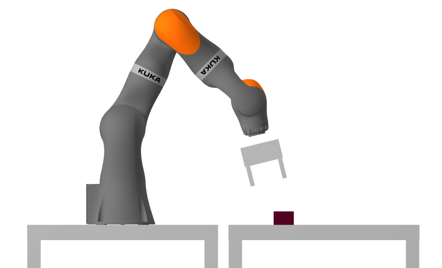
The class starts with a setup that a robotic arm need to pick a brick and place it to a target position. This naturally require many steps including
- Perception
- Kinematics
- Control
- …
For this post, we are starting from kinematics that correspond to Chapter 3. Starting from the notation:
\[^{B}p^{A}\]which usually denotes a point $A$ in frame $B$, for example $^{W}p^A$ is point $A$ position in world frame. Robotic arm typically need many frames described at each motor. Hence, we typically need
\[^{B}p^{A} = X \quad {}^{C}p^{A}\]where $X = {}^{B}X^{C}$ which describe a transformation of a point in frame $C$ converted to frame $B$. For example,
\[^{C}p^{A} = {}^{C}X^{W} \quad {}^{W}p^{A}\]where $C$ is camera frame and ${}^{C}X^{W}$ describes the transformation from world frame to camera frame. $X$ is composed of two components, translation and rotation as shown below
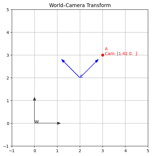
\[\begin{equation*}{}^Gp^A = {}^GX^F {}^Fp^A = {}^Gp^F + {}^Fp^A_G = {}^Gp^F + {}^GR^F {}^Fp^A. \end{equation*}\]where we shall realize that ${}^Gp^F$ can describe a translation vector (as well as a point in a frame). For example, we can illustrate in 2d about the transformation with camera and object.
import numpy as np
import matplotlib.pyplot as plt

# -----------------------------
# Frame Transform (2D or 3D)
# -----------------------------
class FrameTransform:
    def __init__(self, R, t):
        self.R = np.asarray(R)
        self.t = np.asarray(t)
        self.dim = self.R.shape[0]

    @property
    def matrix(self):
        M = np.eye(self.dim + 1)
        M[:self.dim, :self.dim] = self.R
        M[:self.dim, self.dim] = self.t
        return M

    def apply(self, p):
        p_h = np.append(p, 1)
        return (self.matrix @ p_h)[:self.dim]

    def inverse(self):
        R_inv = self.R.T
        t_inv = -R_inv @ self.t
        return FrameTransform(R_inv, t_inv)

# -----------------------------
# Helper: 2D rotation matrix
# -----------------------------
def rot2d(theta_deg):
    th = np.radians(theta_deg)
    c, s = np.cos(th), np.sin(th)
    return np.array([[c, -s], [s, c]])

# -----------------------------
# Example setup
# -----------------------------
W_p_A = np.array([3.0, 3.0])          # Point in World
cam_pos = [2.0, 2.0]                  # Camera position
cam_rot = rot2d(45)                   # Camera rotated 45° in world

W_X_C = FrameTransform(cam_rot, cam_pos)
C_X_W = W_X_C.inverse()

C_p_A = C_X_W.apply(W_p_A)

print("Point A in World:", W_p_A)
print("Point A in Camera:", C_p_A)

# -----------------------------
# Visualization
# -----------------------------
def plot_frame(ax, T, name, color):
    o = T.apply([0, 0])
    x = T.apply([1, 0])
    y = T.apply([0, 1])

    ax.arrow(o[0], o[1], x[0]-o[0], x[1]-o[1], head_width=0.1, fc=color, ec=color)
    ax.arrow(o[0], o[1], y[0]-o[0], y[1]-o[1], head_width=0.1, fc=color, ec=color)
    ax.text(o[0], o[1], name, color=color)

fig, ax = plt.subplots(figsize=(6, 6))

plot_frame(ax, FrameTransform(np.eye(2), [0, 0]), "W", "black")
plot_frame(ax, W_X_C, "C", "blue")

ax.plot(W_p_A[0], W_p_A[1], 'ro')
ax.text(W_p_A[0]+0.1, W_p_A[1],
        f"A\nCam: {C_p_A.round(2)}",
        color='red')

ax.set_aspect('equal')
ax.set_xlim(-1, 5)
ax.set_ylim(-1, 5)
ax.grid(True)
ax.set_title("World–Camera Transform")
plt.show()